The SMPG is a powerful analytical tool designed to monitor the progression of the rainfall season by blending rapidly updated station observations, gridded rainfall data, and forecast information. To ensure seamless integration into existing workflows, the SMPG is designed as a plugin for QGIS. It utilizes time series data extracted for each polygon, making it an intuitive addition to GIS-based monitoring and analysis systems. The SMPG tool is designed to work with the outputs of the GeoCLIM, which is also available as a QGIS plugin. The GeoCLIM can be used to generate Improved Rainfall Estimates (IRE) by blending satellite-based gridded datasets with meteorological station observations. Users can also input time series data into SMPG from their custom workflows.
The SMPG Objective
How the SMPG Works
SMPG Outputs (Products)
The SMPG tool produces two complementary types of products:
1) Map-based outputs (Spatial Summaries)
These products summarize results across all polygons and present them as a set of maps. Each map displays a selected monitoring or outlook indicator for every polygon in the analysis domain, allowing users to quickly identify the status of the season (e.g. below normal, near normal, or above normal, and where probabilities indicate elevated risk).
Common mapped indicators include:
- Current Dekad/LTA Pct.: the percent of average for accumulated precipitation from the Start of Season (SOS) up to the current dekad
- Ensemble Med./LTA Pct.: the percent of the most likely end-of-season outcome relative to the long-term average
- Probability Below Normal: the probability of the season ending below normal (<33rd percentile)
- Probability Normal: the probability of the season ending normal (between the 33rd and 67th percentiles)
- Probability Above Normal: the probability of the season ending above normal (>67th percentile)
- Current Season Pctl.: the percentile rank of accumulated rainfall from SOS up to the current dekad
- Current + Forecast/LTA Pct.: the percent of average seasonal rainfall from SOS to the current dekad including forecast for the next dekad (where available)
Example
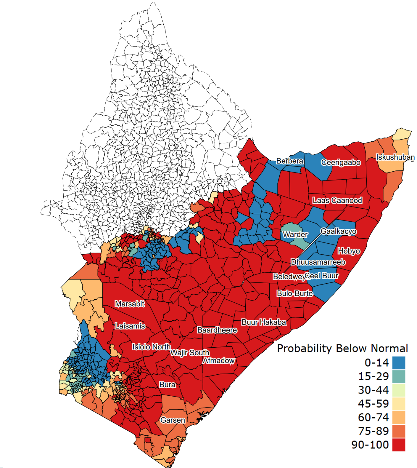 |
Fig. 1. A map of East Africa showing the probability of the 2025 October-December rainfall season ending below normal (left) and IRE seasonal rainfall accumulation in Isiolo North (Kenya) from the start of the season to the November dekad 3 plus forecast (right). The blue bars show the dekadal rainfall accumulation, the red line shows the long term average (LTA) and the purple bar shows the rainfall forecast for the next dekad.
2) Polygon-level plots (detailed diagnostics)
For each polygon, SMPG generates a set of diagnostic plots that explain how the season is evolving from the Start of Season (SOS) to the current time step:
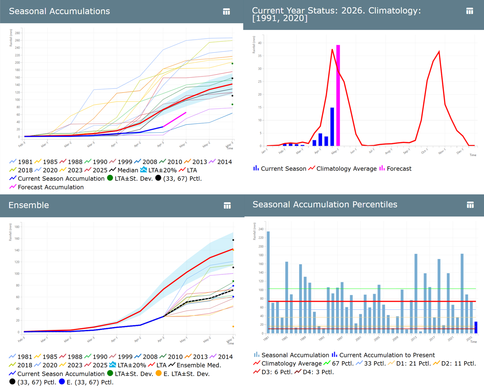
Upper-left plot – Seasonal Accumulations: tracks cumulative rainfall progression against the long-term average (LTA), historical variability, and selected analog years
Upper-right plot – Current Year Status: summarizes the intra-seasonal rainfall distribution and highlights shifts in timing and dry spells relative to the climatological pattern
Lower-left plot – Ensemble: completes the remainder of the season using historical rainfall sequences from the selected analog years (with forecast inputs optional) to generate end-of-season projections, summarize the most-likely outcome, and quantify the probabilities of finishing below normal, near normal, or above normal
Lower-right plot – Seasonal Accumulation Percentiles: places the current season in a historical ranking context using percentile or tercile thresholds to indicate below/near/above-normal conditions
These plots are intended to support agroclimatic decision-making by showing both the current trajectory and the plausible range of end-of-season outcomes for a specific area.
The QGIS SMPG tool plugin and installation guide can be found here.
Video Tutorial: Youtube